c0ldfashioned.net

Introduction

As part of my Summer of Data Science (#SoDS), I knew I wanted to create a project that combined two of my favorite things - baseball and data science! After some searching, I came across a really interesting blog post that used baseball batting averages in an example to illustrate Empirical Bayes methods. This blog post was very thorough in explaining the steps behind the method, using R, a popular software platform used in data science and statistics. Being a Python user, I decided that a good project would be to recreate this exploration using Python. Below, I’ll show you a few of the highlights, and things I learned along the way. You can find the complete jupyter notebook on my GitHub page.

The Data

This project used data from the venerable Lahman database. This database is unbelievably massive. If you read through the jupyter notebook, you’ll see what I mean. TL;DR - each .csv file includes yearly stats from the beginning of baseball’s recorded history! The first step was loading the batting.csv file into a pandas dataframe. After some initial exploratory work, I moved on to the task of whittling down the data, just like the original blog post I am following. First, I created a new column for batting average, calculated as hits (H) divided by at bats (AB). Next, I filtered the dataframe to remove players with fewer than 500 career at bats, in an effort to reduce noise and skew in the resulting histogram, shown below.

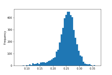
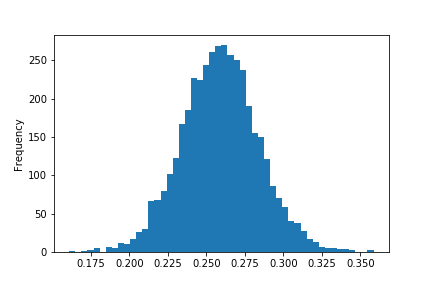
As you can see, there’s still a little bit of skew in the data. Here’s where I found a difference in the data that I used and the data that the original author used. My data still included all pitchers, so the next task was to filter out those players, leaving only those who made their hay with the lumber! The resulting histogram of batting averages now looks like the one in the example project.

Gettin’ Bayesian With It

Bayesian statistics involves the selection of a “prior”, that is, choosing a distribution that we think approximates our data. In this case a beta distribution fits our data rather well. The first step with Empirical Bayes is to estimate a beta prior using the data (hence empirical!). Rather than picking a beta prior randomly, we use historical data to establish our beta prior. Estimating the beta prior from the data works particularly well when there is a lot of data to work with - perfect for our massive dataset from baseball history. After much googling and stack overflowing (yes, those are verbs to me!), I found that you can use scipy to get the relevant beta distribution values, namely $\alpha_o$ and $\beta_o$. It turned out to be easier than I expected to get those values - it took all of three lines of code, seen here:

from scipy.stats import beta
data = list(no_pitchers['Avg'])
alpha0, beta0, _, __ = beta.fit(data, floc=0, fscale=1)

Now that we have estimated our beta prior, plotting it on top of the histogram of the data we used looks like this: Not too bad, eh? The red line is our beta prior, based on the data represented by the histogram. For reference, here’s the code that created the above chart.

fig, ax = plt.subplots(1,1,figsize=(6,4))
x = np.linspace(beta.ppf(0.001, alpha0, beta0),
               beta.ppf(0.999, alpha0, beta0))
ax.plot(x, beta.pdf(x, alpha0, beta0), 'r-', label='beta pdf')
no_pitchers.Avg.plot.hist(bins=50, normed=True)
plt.show()

Ok, now what? (aka, Get On With It!)

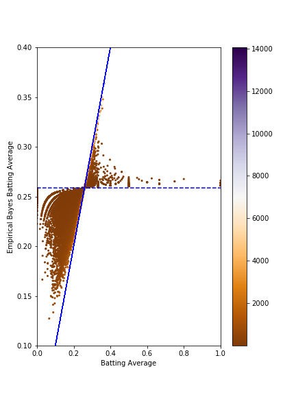
If I understand the example project I followed, the beta prior values of alpha0 and beta0 are combined with new data resulting in an estimate for future behavior that is tempered, so to speak. That is, the beta prior developed from historic data has the effect of “shrinking” new data toward the historical results. This behavior is useful for things like baseball statistics, due to the rich history of collecting stats. The other benefit to working with an empirically derived beta prior is that it minimizes the affect of cases with fewer examples (0-for-1, or 1-for-1) on our estimates. In a sense, it gives more weight to examples of large size (more career at bats). I applied the beta prior values to the entire batting dataset (no players excluded), creating an estimate of batting average as influenced by the beta prior from the subset of hitters that was developed. Below is a plot of all players’ estimated batting average vs. their actual career batting average. I’m still wrapping my head around this plot, but it’s visually impressive, and fairly intuitive. The horizontal dashed line represents what our model would estimate for any given hitter with no actual data to work with. The diagonal line is y=x, which shows that our estimates match up well with the players who have the largest amount of at bats. i.e. points close to this line were not influenced as strongly by the beta prior compared to points farther away from this line.

Wrapping Up

This is just one example of how Empirical Bayes can be applied to baseball statistics. I found this project really interesting, and since it was written in R, set a goal to recreate it in Python. I definitely enjoyed the work and learned a lot about pandas and matplotlib along the way. I’m looking forward to applying this technique to more aspects of the Lahman database and seeing what other insights could be gained. If you made it this far, thanks for reading, I hope you found something interesting, or even insightful. However, it’s also OK if you just liked the charts - I know I did.